Particle data in VTK XML

In my previous post on writing VTK output files I described how mesh data can be output in VTK XML format. In this article I will talk about how I output particle data from my simulations.

These simulations use a number of techniques depending on the requirements. I use the MPM (Material Point Method) and RBD (Rigid body dynamics) with the occasional DEM (Discrete/Distict element method) and Peridynamics simulation. When I am running RBD or DEM simulations, the particles may have not spherical shapes and the shape and orientation information have to be encoded into the output data in addition to other physical state variables.

Note: The visualization of non-spherical particles in Visit/Paraview requires the implementation of a plugin that can perform the appropriate transformation. Alternatively, we can convert each particle into a surface mesh before writing the output. We will not discuss these issues at this stage. However, in future posts we will show how these plots can be generated using Javascript.

Particle data

We will assume that the particles are ellipsoids. The particle data that we will output in this example are:

• The particle ID
• The particle radii in the three principal axis directions
• The three principal axis orientations
• The particle position
• The particle velocity

Writing the particle data

To write the particles data to the disk, we follow the same approach as we did for the grid/mesh data in the previous post. The writeParticles function has the form

void
OutputVTK::writeParticles(double time,
                          const ParticlePArray* particles,
                          std::ostringstream& fileName)
{
  // Create a writer
  auto writer = vtkXMLUnstructuredGridWriterP::New();
  // Get the filename with extension
  fileName << "." << writer->GetDefaultFileExtension();
  writer->SetFileName((fileName.str()).c_str());
  // Create a pointer to a VTK Unstructured Grid data set
  auto dataSet = vtkUnstructuredGridP::New();
  // Set up pointer to point data
  auto pts = vtkPointsP::New();
  // Count the total number of points
  int num_pts = static_cast<int>(particles->size());
  pts->SetNumberOfPoints(num_pts);
  // Add the time
  addTimeToVTKDataSet(time, dataSet);
  // Add the particle data to the unstructured grid
  addParticlesToVTKDataSet(particles, pts, dataSet);
  // Set the points
  dataSet->SetPoints(pts);
  // Remove unused memory
  dataSet->Squeeze();
  // Write the data
  writer->SetInput(dataSet);
  writer->SetDataModeToBinary();
  writer->Write();
}

We have already seen the addTimeToVTKDataSet method in the previous post. The main difference in this case is the new addParticlesToVTKDataSet method:

void
OutputVTK::addParticlesToVTKDataSet(const ParticlePArray* particles,
                                    vtkPointsP& pts,
                                    vtkUnstructuredGridP& dataSet)
{
  // Set up pointers for material property data
  auto ID = vtkDoubleArrayP::New();
  ID->SetNumberOfComponents(1);
  ID->SetNumberOfTuples(pts->GetNumberOfPoints());
  ID->SetName("ID");

  auto radii = vtkDoubleArrayP::New();
  radii->SetNumberOfComponents(3);
  radii->SetNumberOfTuples(pts->GetNumberOfPoints());
  radii->SetName("Radius");

  auto axis_a = vtkDoubleArrayP::New();
  axis_a->SetNumberOfComponents(3);
  axis_a->SetNumberOfTuples(pts->GetNumberOfPoints());
  axis_a->SetName("Axis a");

  auto axis_b = vtkDoubleArrayP::New();
  vtkDoubleArrayP axis_b = vtkDoubleArrayP::New();
  axis_b->SetNumberOfComponents(3);
  axis_b->SetNumberOfTuples(pts->GetNumberOfPoints());
  axis_b->SetName("Axis b");

  auto axis_c = vtkDoubleArrayP::New();
  axis_c->SetNumberOfComponents(3);
  axis_c->SetNumberOfTuples(pts->GetNumberOfPoints());
  axis_c->SetName("Axis c");

  auto position = vtkDoubleArrayP::New();
  position->SetNumberOfComponents(3);
  position->SetNumberOfTuples(pts->GetNumberOfPoints());
  position->SetName("Position");

  auto velocity = vtkDoubleArrayP::New();
  velocity->SetNumberOfComponents(3);
  velocity->SetNumberOfTuples(pts->GetNumberOfPoints());
  velocity->SetName("Velocity");

  // Loop through particles
  Vec vObj;
  int id = 0;
  double vec[3];
  for (const auto& particle : *particles) {

    // Position
    vObj = particle->getCurrPos();
    vec[0] = vObj.getX();
    vec[1] = vObj.getY();
    vec[2] = vObj.getZ();
    pts->SetPoint(id, vec);

    // ID
    ID->InsertValue(id, particle->getId());

    // Ellipsoid radii
    vec[0] = particle->getA();
    vec[1] = particle->getB();
    vec[2] = particle->getC();
    radii->InsertTuple(id, vec);

    // Current direction A
    vObj = particle->getCurrDirecA();
    vec[0] = vObj.getX();
    vec[1] = vObj.getY();
    vec[2] = vObj.getZ();
    axis_a->InsertTuple(id, vec);

    // Current direction B
    vObj = particle->getCurrDirecB();
    vec[0] = vObj.getX();
    vec[1] = vObj.getY();
    vec[2] = vObj.getZ();
    axis_b->InsertTuple(id, vec);

    // Current direction C
    vObj = particle->getCurrDirecC();
    vec[0] = vObj.getX();
    vec[1] = vObj.getY();
    vec[2] = vObj.getZ();
    axis_c->InsertTuple(id, vec);

    // Velocity
    vObj = particle->getCurrVeloc();
    vec[0] = vObj.getX();
    vec[1] = vObj.getY();
    vec[2] = vObj.getZ();
    velocity->InsertTuple(id, vec);
    
    ++id;
  }

  // Add points to data set
  dataSet->GetPointData()->AddArray(ID);
  dataSet->GetPointData()->AddArray(radii);
  dataSet->GetPointData()->AddArray(axis_a);
  dataSet->GetPointData()->AddArray(axis_b);
  dataSet->GetPointData()->AddArray(axis_c);
  dataSet->GetPointData()->AddArray(velocity);
}

You can see a working example of this approach in the Matiti code.

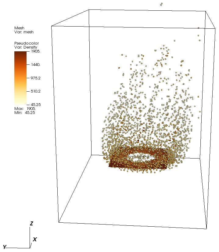
Displaying the output

The VTK XML file output to disk using this approach can be visualized in Visit or ParaView. Notice that we are not able to use the particle geometry and orientation information in either of these tools without extra work. The plot below shows the output of a rigid body dynamics simulation in the presence of Coriolis forces.

Remarks

Now that the basic input/output issues have been addressed, we will be able to explore possible designs of an integrated user interface to automate the generation of input files and perform simple visualizations of the results. Future blog posts will discuss our exploration of Javascript frameworks and libraries that can potentially aid this process.