Meshes with different element topologies in gmsh (for Code-Aster)

38 minute read

We have been translating a few Code-Aster verification test manuals into English. The process is not just a straightforward translation of the text in the French manuals. We also annotate the command files during the process and try to generate new meshes when the task is not too difficult. Sometimes Salome-Meca is more convenient for mesh generation. At other times we choose to use gmsh.

Recently, during the process of translation the manual for the SSNV112 tests, we realized that we needed meshes containing HEXA20, PENTA15, TETRA10, QUAD8, and TRIA6 elements instead on the complete elements HEXA27, PENTA18, TETRA10, QUAD9, and TRIA6 that are generated by gmsh under default conditions.

In this article, we will discuss the options that can be used in gmsh to create meshes containing these elements. We will also talk a bit about how the element numbers that are associated with the keyword MAILLE in Code_Aster can be identified in the gmsh meshes.

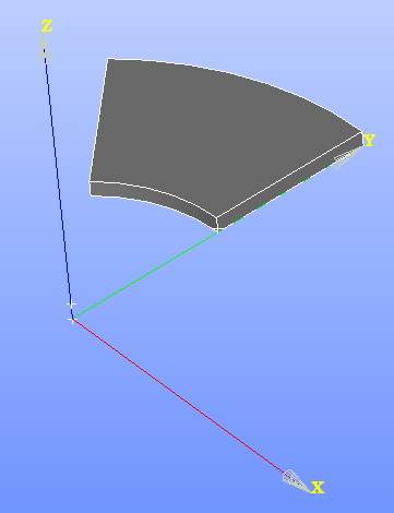
Geometry of the segment of the cylinder to be meshed.

The geometry

The model consists a hollow circular cylinder that is modeled as a 45 degree segment as shown in the figure.

We want to mesh this geometry using:

20-node hexahedral elements
15-node prism elements
10-node tetrahedral elements
a mix of 8-node quarilaterals and 6-node triangle elements

We also want to retain the general properties of the meshes provided with the Code_Aster validation test suite; the meshes that we create with gmsh have to be similar to those in the test suite.

Setting up `gmsh` for modeling and meshing

We will use the Python interface to gmsh and use Juypter notebook to make the process of mesh generation reasonably interactive. To do that we set up a Python3 environment and install gmsh into it using pip. Once inside the interactive environment:

First, we will import the packages we will need:

import gmsh
import sys
import math
import json

Then we will initialize gmsh. We will use the OpenCascade kernel to create and mesh the geometry.

 # Initialize gmsh
 gmsh.initialize()

 # Choose kernel
 model = gmsh.model
 occ = model.occ
 mesh = model.mesh
 model.add("ssnv112a")

We will then create the plane geometry for the models

# Geometry parameters
RI = 0.1
RE = 0.2
NR = 12
NT = 10
NZ = 2
H = 0.01

# Add points
PO = occ.addPoint(0.,  0.,  0., el_size)
POP = occ.addPoint(0.,  0.,  H, el_size)
A = occ.addPoint(0.,  RI,  0., el_size)
B = occ.addPoint(0.,  RE,  0., el_size)
E = occ.addPoint((RI*(2. ** 0.5)/(-2.)), (RI*(2. ** 0.5)/2.),  0., el_size) 
F = occ.addPoint((RE*(2. ** 0.5)/(-2.)), (RE*(2. ** 0.5)/2.),  0., el_size) 
node_mid = occ.addPoint(0., RI, (H/NZ/2.), el_size)

# Add lines and arcs
LAB = occ.addLine(A, B)
LBF = occ.addCircleArc(B, PO, F)
LFE = occ.addLine(F, E)
LEA = occ.addCircleArc(E, PO, A)

# Add curve loop and plane surface
FACINF_loop = occ.addCurveLoop([LAB, LBF, LFE, LEA])
FACINF = occ.addPlaneSurface([FACINF_loop]) 

We will then create 3D models, if necessary. Some minor differences exist between models which will be discussed later.
The geoemtry will then be synchronized in gmsh.
```
occ.synchronize()
```

Physical groups needed in the Code_Aster computation will then be added.

# Physical groups for the points
A_g = model.addPhysicalGroup(0, [A])
model.setPhysicalName(0, A_g, 'A')
B_g = model.addPhysicalGroup(0, [B])
model.setPhysicalName(0, B_g, 'B')
E_g = model.addPhysicalGroup(0, [E])
model.setPhysicalName(0, E_g, 'E')
F_g = model.addPhysicalGroup(0, [F])
model.setPhysicalName(0, F_g, 'F')
AP_g = model.addPhysicalGroup(0, [7])
model.setPhysicalName(0, AP_g, 'AP')
EP_g = model.addPhysicalGroup(0, [10])
model.setPhysicalName(0, EP_g, 'EP')
nodemid_g = model.addPhysicalGroup(0, [node_mid])
model.setPhysicalName(0, nodemid_g, 'NOEUMI')
  
# Physical groups for the edges
LAB_g = model.addPhysicalGroup(1, [LAB])
model.setPhysicalName(1, LAB_g, 'LAB')
LBF_g = model.addPhysicalGroup(1, [LBF])
model.setPhysicalName(1, LBF_g, 'LBF')
LFE_g = model.addPhysicalGroup(1, [LFE])
model.setPhysicalName(1, LFE_g, 'LFE')
LEA_g = model.addPhysicalGroup(1, [LEA])
model.setPhysicalName(1, LEA_g, 'LEA')
  
# Physical groups for the faces
FACEAB_g = model.addPhysicalGroup(2, [2])
model.setPhysicalName(2, FACEAB_g, 'FACEAB')
FACEAE_g = model.addPhysicalGroup(2, [5])
model.setPhysicalName(2, FACEAE_g, 'FACEAE')
FACSUP_g = model.addPhysicalGroup(2, [6])
model.setPhysicalName(2, FACSUP_g, 'FACSUP')
FACEEF_g = model.addPhysicalGroup(2, [4])
model.setPhysicalName(2, FACEEF_g, 'FACEEF')
FACINF_g = model.addPhysicalGroup(2, [FACINF])
model.setPhysicalName(2, FACINF_g, 'FACINF')
  
# Physical group for the volume
VOLUME_g = model.addPhysicalGroup(3, [1])
model.setPhysicalName(3, VOLUME_g, 'VOLUME')

If regular meshes are desired, we may need to set up transfinite interpolation:

num_nodes = NT+1
for curve in [2, 4, 9, 12]:
    mesh.setTransfiniteCurve(curve, num_nodes)
num_nodes = NR+1
for curve in [1, 3, 7, 11]:
    mesh.setTransfiniteCurve(curve, num_nodes)
num_node = NZ+1
for curve in [5, 6, 8, 10]:
    mesh.setTransfiniteCurve(curve, num_nodes)
  
for surf in occ.getEntities(2):
    mesh.setTransfiniteSurface(surf[1])
  
for vol in occ.getEntities(3):
    mesh.setTransfiniteVolume(vol[1])

The we will specify meshing options:

gmsh.option.setNumber('Mesh.RecombineAll', 1)
gmsh.option.setNumber('Mesh.RecombinationAlgorithm', 1)
gmsh.option.setNumber('Mesh.Recombine3DLevel', 2)
gmsh.option.setNumber('Mesh.ElementOrder', 2)
gmsh.option.setNumber('Mesh.MshFileVersion', 2.2)
gmsh.option.setNumber('Mesh.MedFileMinorVersion', 0)
gmsh.option.setNumber('Mesh.SaveAll', 0)
gmsh.option.setNumber('Mesh.SaveGroupsOfNodes', 1)
gmsh.option.setNumber('Mesh.SecondOrderIncomplete', 1)

Finally, we generate and save the mesh:

# Generate mesh
mesh.generate(3)
mesh.recombine()

# Save mesh
gmsh.write("ssnv112a_upd.med")

To visualize the data, we use:
```
gmsh.fltk.run()
```
To cleanly exit the gmsh engine, we wrap up the run with
```
gmsh.finalize()
```

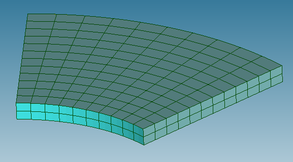
20-node hexahedra (`HEXA20`)

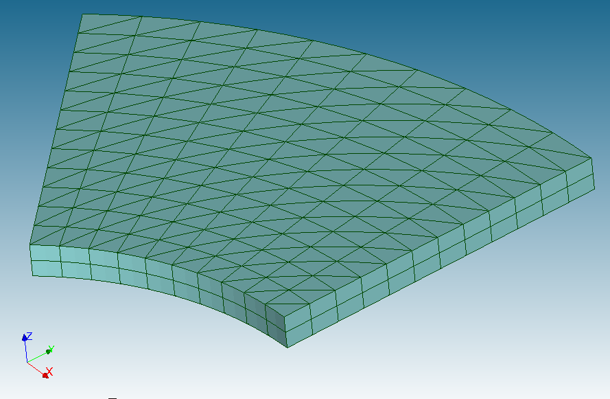
The HEAX20 mesh provided by Code_Aster is shown in the adjacent figure. We can see that the mesh has two elements through the thickness, 12 elements in the radial direction, and 10 elements in the circumferential direction.

To create a similar mesh with gmsh, we have to use transfinite interpolation and then use the recombine feature to create hexahedral elements.

To set up the model for recombination, we extrude the plane geometry created in the previous section with a recombine = True flag and with NZ = 2 elements through the thickness:
```
 # Create volume by extrusion
 VOLUME = occ.extrude([(2, FACINF)], 0., 0., H, [NZ], recombine=True)
```
We use the transfinite interpolation commands in the previous section. Note that we could alternatively have extruded the mesh directly (as we will shown for the PENTA15 case).
To make sure that 20-node hexahedra are generated (instead of 27-node hexahedra), we use the flag
```
 gmsh.option.setNumber('Mesh.SecondOrderIncomplete', 1)
```

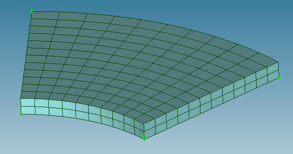
The mesh created by gmsh is show in the adjacent figure. Note that it is almost identical to that provided by gmsh.

To generate tetrahedral meshes containing 10-node elements (TETRA10) from the same geometry, we have to turn a few options off. We no longer need mesh.setTransfiniteVolume(...) and mesh.recombine(), or to set the option Mesh.RecombineAll.

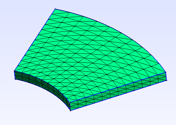
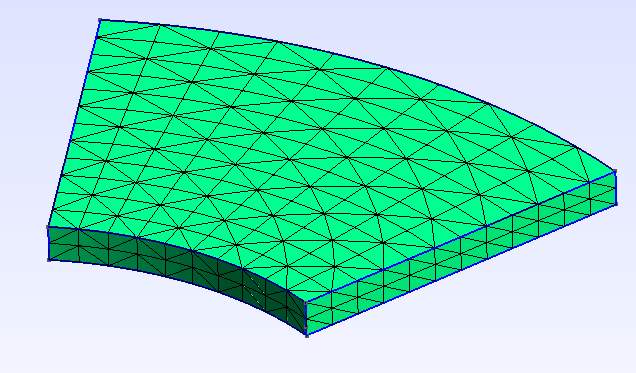
TETRA10 meshes generated by gmsh. (a) with transfinite interpolation of the curves and surfaces. (b) transfinite interpolation of curves and surface with Alternate flag. (c) no transfinite interpolation.

If we retain transfinite curves and surfaces, the tetrahedral mesh that is generated has a bias as can be seen in figure (a) above. The bias can be removed with the Alternate flag:

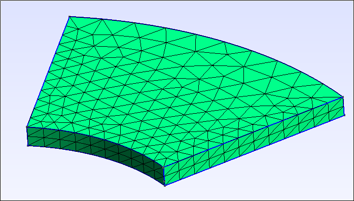
mesh.setTransfiniteSurface(surf[1], arrangement='Alternate')

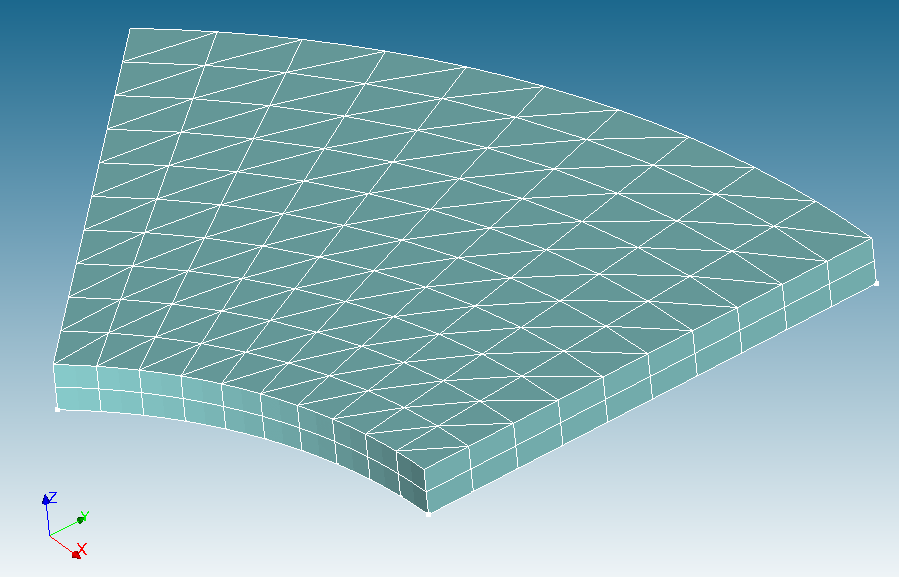
The resulting mesh can be seen in the middle figure (b) above. If we turn off transfinite interpolation, we get an unordered tetrahedral mesh as see in figure (c) above.

15-node prism (`PENTA15`) elements

The mesh provided by Code_Aster is shown in the adjacent figure. Note that the top and bottom faces have triangular facets while the sides have quadrilateral facets.

Before generating this mesh, as before, we set up the geometry using extrusion with the recombine = True flag using two elements through the thickness.

# Surfaces
tri_loop = occ.addCurveLoop([LAB, LBF, LFE, LEA])
tri = occ.addPlaneSurface([tri_loop])

# Volume
vol = occ.extrude([(2, tri)], 0, 0, h, [2], recombine = True)

We also set up transfinite interpolation for the surface that is extruded:

num_nodes = NT+1
for curve in [LBF, LEA]:
    mesh.setTransfiniteCurve(curve, num_nodes)
num_nodes = NR+1
for curve in [LAB, LFE]:
    mesh.setTransfiniteCurve(curve, num_nodes)

mesh.setTransfiniteSurface(tri)

However, we no longer need transfinite interpolation through the thickness. We also don’t need recombination.

Nevertheless, to avoid generating complete prism elements, we do need

gmsh.option.setNumber('Mesh.SecondOrderIncomplete', 1)

The mesh generated by this process is shown in the adjacent figure. It is almost identical to that provided by Code_Aster. However, the number of nodes and elements are slightly different.

Mix of 8-node quadrilateral (`QUAD8`) and 6-node triangle (`TRIA6`) elements

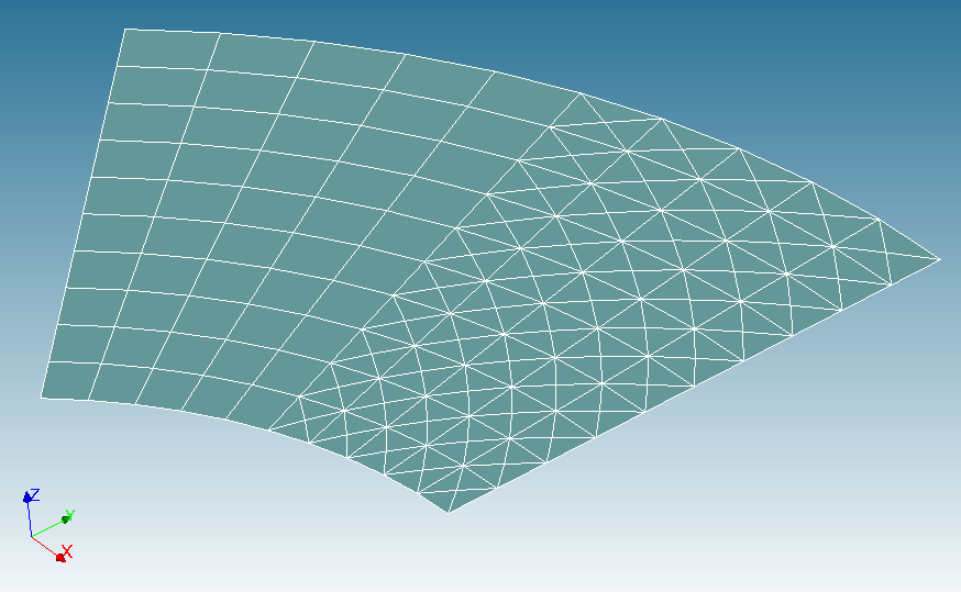
QUAD8/TRIA6 mixed mesh provided by Code_Aster.

The adjacent figure show the 2D mesh of mixed quadrilateral/triangle elements provide in the Code_Aster validation suite.

To generate such a mesh with gmsh, we have to partition the geometry into two areas:

# Geometry
ri=0.1
re=0.2
c225 = np.cos(22.5*math.pi/180)
s225 = np.sin(22.5*math.pi/180)
NR = 10
NT = 5

# Default element size
dens = 0.01;

# Points of construction
PO = occ.addPoint(0, 0, 0,  dens)

# Points of the plane of the base z=0
A = occ.addPoint(0, ri, 0., dens)
B = occ.addPoint(0, re, 0., dens)
C = occ.addPoint(-ri * s225, ri * c225, 0, dens)
D = occ.addPoint(-re * s225, re * c225, 0, dens)
E = occ.addPoint(-(ri/(2 ** 0.5)) , (ri/(2 ** 0.5)), 0.,  dens)
F = occ.addPoint(-re/(2 ** 0.5) , re/(2 ** 0.5) , 0.,  dens)

# Lines
LAB = occ.addLine(A, B)
LBD = occ.addCircleArc(B, PO, D)
LDC = occ.addLine(D, C)
LCA = occ.addCircleArc(C, PO, A)

LDF = occ.addCircleArc(D, PO, F)
LFE = occ.addLine(F, E)
LEC = occ.addCircleArc(E, PO, C)

# Surfaces
tri_loop = occ.addCurveLoop([LAB, LBD, LDC, LCA])
tri = occ.addPlaneSurface([tri_loop])
quad_loop = occ.addCurveLoop([-LDC, LDF, LFE, LEC])
quad = occ.addPlaneSurface([quad_loop])

occ.synchronize()

The edges are set to transfinite as before:

num_nodes = NT+1
for curve in [LCA, LEC, LBD, LDF]:
    #print(curve)
    mesh.setTransfiniteCurve(curve, num_nodes)
num_nodes = NR+1
for curve in [LAB, LFE]:
    #print(curve)
    mesh.setTransfiniteCurve(curve, num_nodes)

However, to match the lack of bias in the triangles in the Code_Aster mesh, we need to add the Alternate flag while flagging the transfinite surfaces

for surf in occ.getEntities(2):
    mesh.setTransfiniteSurface(surf[1], arrangement='AlternateRight')

An important step at this stage to to set recombination on for the area that is to be meshed with quadrilateral elements:

mesh.setRecombine(2, quad)

Also, to make sure that QUAD9 elements are not generated instead of QUAD8, we need

gmsh.option.setNumber('Mesh.SecondOrderIncomplete', 1)

Finally, since we only need a 2D mesh, we run

mesh.generate(2)

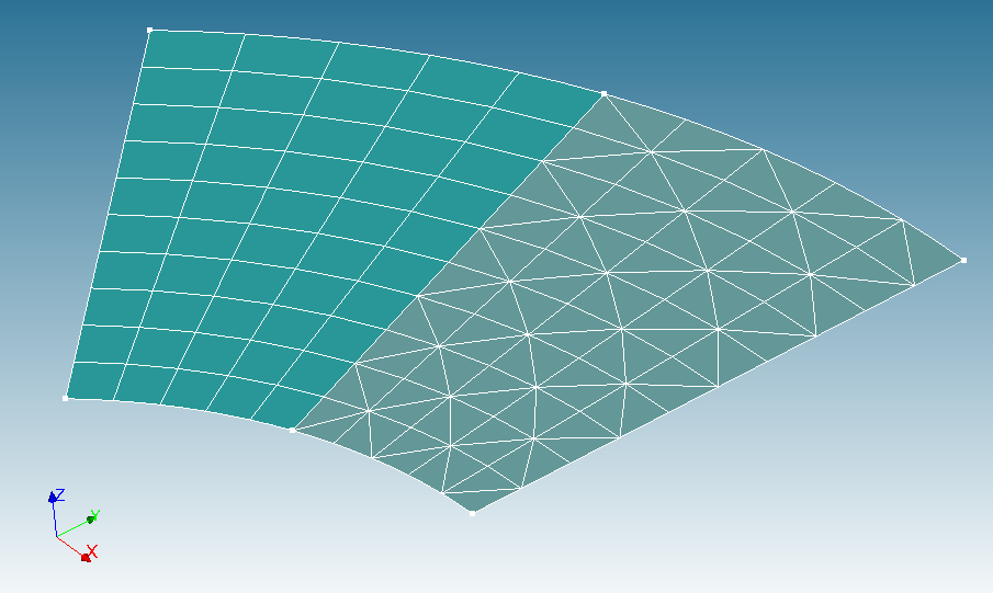
QUAD8/TRIA6 mixed mesh generated by gmsh (compare with that provided by Code_Aster).

The mesh created by gmsh appears to have a less dense distribution of triangles than that provided by Code_Aster. That is because gmsh does not allow the creation of cross-hatch elements. It is not clear how the two meshes can be made identical. However, for the purposes of verification, the differences between the two meshes appear not to matter much.

Identifying specific elements in `Code_Aster` command files

The original verification tests contain hard-coded element numbers (MAILLE = xx) that are no longer valid when the mesh is changed. Also, the MAILLE tag has been deprecated. We would like to replace these with appropriate element groups (GROUP_MA).

The first step in the process is to convert the mesh files (typically in MED format) into ASTER text format.

DEBUT(LANG='EN')
mesh = LIRE_MAILLAGE(FORMAT='MED',
                     UNITE=20)
IMPR_RESU(FORMAT='ASTER',
          RESU=_F(MAILLAGE=mesh),
          UNITE=80)
FIN()

The output file can then be used to identify the elements which have been referred to in the verification command files and the element groups can be chosen accordingly.

Also, the output mesh file from gmsh does not contain any node groups. These have to be generated from saved 0D element groups (point physical groups in gmsh).

Model A (HEXA20 elements)

In the case of MODEL A (SSNV112A), we need node groups for points A, E, F, and an element group for element M1. These are created using DEFI_GROUP.

The node groups are created using

# Define node groups
mesh = DEFI_GROUP(reuse = mesh,
                  MAILLAGE = mesh,
                  CREA_GROUP_NO = (_F(GROUP_MA = ('A', 'E', 'F'))))

From the ASTER format mesh file, the element M1 is found to be the one that contains point A. We can use a ball around A to find the element which belongs to this group. Th radius is chosen so that we select only one element:

# Define element groups
mesh = DEFI_GROUP(reuse = mesh,
                  MAILLAGE = mesh,
                  CREA_GROUP_MA = (_F(NOM = 'M1',
                                      TYPE_MAILLE = '3D',
                                      OPTION = 'SPHERE',
                                      GROUP_NO_CENTRE = 'A',
                                      RAYON = 0.002)))

Model B (TETRA10 elements)

Finding the element groups for Model B (SSNV112B) is a bit more involved because all nodes are shared by multiple elements.

As before, we extract the mesh in an ASTER format file and note that element M537 is attached to nodes A, N48, N84, and N362.

First we create node groups for these nodes:

# Define node groups
mesh = DEFI_GROUP(reuse = mesh,
                  MAILLAGE = mesh,
                  CREA_GROUP_NO = (_F(GROUP_MA = 'A',
                                      NOM = 'A'),
                                   _F(GROUP_MA = 'F',
                                      NOM = 'F'),
                                   _F(NOM = 'N48',
                                      OPTION = 'ENV_SPHERE',
                                      POINT = (9.93712209893243E-02,  1.11964476103304E-02,  0.00000000000000E+00),
                                      RAYON = 0.002,
                                      PRECISION = 0.001),
                                   _F(NOM = 'N84',
                                      OPTION = 'ENV_SPHERE',
                                      POINT = (9.93712209893243E-02,  1.11964476103307E-02,  1.00000000000000E-02),
                                      RAYON = 0.002,
                                      PRECISION = 0.001),
                                   _F(NOM = 'N362',
                                      OPTION = 'ENV_SPHERE',
                                      POINT = (1.03360166268687E-01,  5.80458243110394E-03,  5.00000000000017E-03),
                                      RAYON = 0.002,
                                      PRECISION = 0.001)))

Next we define element groups for the elements attached to these nodes:

# Define element groups
mesh = DEFI_GROUP(reuse = mesh,
                  MAILLAGE = mesh,
                  CREA_GROUP_MA = (_F(NOM = 'M1',
                                      TYPE_MAILLE = '3D',
                                      OPTION = 'SPHERE',
                                      GROUP_NO_CENTRE = 'A',
                                      RAYON = 0.005),
                                   _F(NOM = 'M2',
                                      TYPE_MAILLE = '3D',
                                      OPTION = 'SPHERE',
                                      GROUP_NO_CENTRE = 'N48',
                                      RAYON = 0.005),
                                   _F(NOM = 'M3',
                                      TYPE_MAILLE = '3D',
                                      OPTION = 'SPHERE',
                                      GROUP_NO_CENTRE = 'N84',
                                      RAYON = 0.005),
                                   _F(NOM = 'M4',
                                      TYPE_MAILLE = '3D',
                                      OPTION = 'SPHERE',
                                      GROUP_NO_CENTRE = 'N362',
                                      RAYON = 0.005)))

To get the unique element that is shared by these groups, we then perform an intersection operation to define the element group M537:

mesh = DEFI_GROUP(reuse = mesh,
                  MAILLAGE = mesh,
                  CREA_GROUP_MA = (_F(NOM = 'M537',
                                      INTERSEC = ('M1', 'M2', 'M3', 'M4'))))

The DEFI_GROUP operations can be very useful when element groups are needed for a calculation but we only have access to a mesh and not its associated geometry.

Remarks

This article discusses ways of generating various types of meshes with gmsh. These tips can be useful for situations such as contact, where standard tetrahedral meshes may not be adequate for convergence.

The addition of element and node groups to meshes using selection criteria in Code_Aster is also a very useful tool for situations where new meshes cannot be generated easily but new physical groups are needed for extraction of results or the application of new boundary conditions.

Share on

Twitter Facebook LinkedIn

Biswajit Banerjee

Meshes with different element topologies in gmsh (for Code-Aster)

The geometry

Setting up `gmsh` for modeling and meshing

20-node hexahedra (`HEXA20`)

15-node prism (`PENTA15`) elements

Mix of 8-node quadrilateral (`QUAD8`) and 6-node triangle (`TRIA6`) elements

Identifying specific elements in `Code_Aster` command files

Model A (HEXA20 elements)

Model B (TETRA10 elements)

Remarks

Share on

You may also enjoy

Creating quadrilateral surface meshes with gmsh

Inspecting and manipulating meshes in Salome-Meca for Code-Aster

Compiling and running the MPM code Vaango on a Cray

Unit testing with MPI, googletest, and cmake

Biswajit Banerjee

The geometry

Setting up gmsh for modeling and meshing

20-node hexahedra (HEXA20)

15-node prism (PENTA15) elements

Mix of 8-node quadrilateral (QUAD8) and 6-node triangle (TRIA6) elements

Identifying specific elements in Code_Aster command files

Model A (HEXA20 elements)

Model B (TETRA10 elements)

Remarks

Share on

You may also enjoy

Creating quadrilateral surface meshes with gmsh

Inspecting and manipulating meshes in Salome-Meca for Code-Aster

Compiling and running the MPM code Vaango on a Cray

Unit testing with MPI, googletest, and cmake

Setting up `gmsh` for modeling and meshing

20-node hexahedra (`HEXA20`)

15-node prism (`PENTA15`) elements

Mix of 8-node quadrilateral (`QUAD8`) and 6-node triangle (`TRIA6`) elements

Identifying specific elements in `Code_Aster` command files