Creating quadrilateral surface meshes with gmsh

The Code-Aster cooling tower modal analysis validation test FORMA11c comes with a quadrilateral mesh provided by Code-Aster.
Tips on quadrilateral meshing with gmsh are sparsely distributed on the open web. In this article, I will discuss how we can recreate the Code-Aster mesh with gmsh.

Mesh provided with Code-Aster.

Extracting the geometry

The first step in the process is to extract the profile of the cooling tower using the Mesh module of Salome-Meca.

To do that, we could pick points along the profile manually but that gets tedious and error-prone quite rapidly as the number of nodes increases. We will use Python scripting instead.

• Read the mesh:

   # Read mesh
   ([mesh], status) = smesh.CreateMeshesFromMED(r'/home/Salome/forma11/forma11c.mmed')
  

• Create a selection box for points on the profile. We want points that are on one of the vertical edges of the cooling tower. We choose points that are between \((0, x_{\text{max}})\) and \((z_{\text{min}}, z_{\text{max}})\) with a small buffer \(\epsilon\) :

   # Create selection box
   eps = 1.0e-3
   mesh_bb = mesh.BoundingBox()
   x_min = 0
   x_max = mesh_bb[3] + eps
   z_min = mesh_bb[2] - eps
   z_max = mesh_bb[5] + eps
   y_min = -eps
   y_max =  eps
  
   box_min = geompy.MakeVertex(x_min, y_min, z_min)
   box_max = geompy.MakeVertex(x_max, y_max, z_max)
   box = geompy.MakeBoxTwoPnt(box_min, box_max)
   geompy.addToStudy(box, "selection_box")
  

• Use a filter to select nodes inside the selection box

   # Get the nodes that are in the selection box
   filter = smesh.GetFilter(SMESH.NODE,  SMESH.FT_BelongToGeom, box)
   ids = mesh.GetIdsFromFilter(filter)
  

• Next we extract the nodal coordinates and add them to a group:

   # Create a node group called "profile" 
   profile = mesh.CreateEmptyGroup( SMESH.NODE, 'profile' )
  
   # Get the nodal coordinates
   coords = []
   for id in ids:
      coords.append(mesh.GetNodeXYZ(id))
  
      # Add the node to the "profile" group
      nbAdd = profile.Add([id])
  

• Finally, save the coordinates to a JSON file. We are using this format because we intend to use the Python interface for gmsh and it is easier to read JSON objects directly with Python.

   # Save the coordinates (json)
   ExportPATH="/home/Salome/forma11/"
   file_id = open( r''+ExportPATH+'forma11c_profile.json'+'', 'w')
   json.dump(coords, file_id)
   file_id.close()
  

Now that we have saved the profile, it’s time to move to gmsh are explore meshing.

Geometry with gmsh

The process of creating and meshing the geometry is easier to iterate upon inside a Jupyter notebook running Python 3.

• First, we import the packages we will need:

  import gmsh
  import sys
  import math
  import json
  

• Then we initialize gmsh. We will use the OpenCascade kernel to create and mesh the cooling tower geometry to take advantage of functions that can be used to select geometrical entities.

  # Initialize gmsh
  gmsh.initialize()
  
  # Choose kernel
  model = gmsh.model
  occ = model.occ
  mesh = model.mesh
  model.add("forma11c_gmsh")
  

• Next we read in the coordinates of the profile from the JSON file we had created in Salome-Meca:

  # Read the profile coordinates
  file_id = open( r''+ExportPATH+'forma11c_profile.json'+'', 'r')
  coords = json.load(file_id)
  file_id.close()
  

Adding the profile points to gmsh

Now that we have the environment ready and the data read from file, we can start creating the geometry in gmsh.

Add the profile points using

# Set a default element size
el_size = 1.0

# Add profile points
v_profile = []
for coord in coords:
    v = occ.addPoint(coord[0], coord[1], coord[2], el_size)
    v_profile.append(v)

We can check that the points are reasonable by using to open the GUI after updating the objects.

occ.synchronize()
gmsh.fltk.run()

Profile points added to `gmsh`.

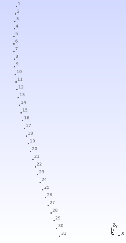
You will see a set of points as shown in the image on the right.

Don’t forget to clean-up after closing the gmsh GUI with gmsh.finalize(). After you do that, you’ll have to rerun the previous steps again to create a clean data set.

Fit a spline through the points

After the points have been added to the OpenCascade model, you will have to create a line that interpolates the points.

We do that in gmsh with the command addBSpline (the special features of this command in the OpenCascade kernel are another reason to use this kernel instead of the built-in geo kernel.

# Add spline going through profile points
l1 = occ.addBSpline(v_profile)

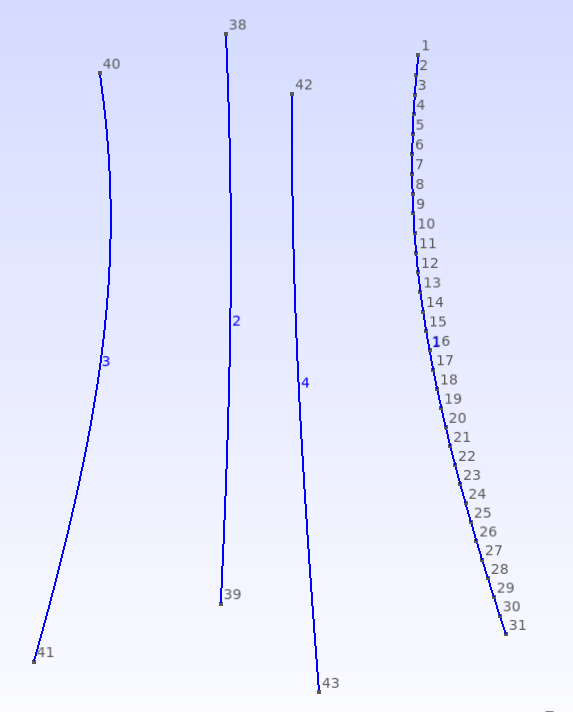
Create copies of the line and rotate them

Because the gmsh sweep function limits the sweep angle, we will create three copies of the line and move them to different positions around the circumference of the cooling tower.

This copying and rotation can be achieved with:

# Create copies and rotate
l2 = occ.copy([(1,l1)])
l3 = occ.copy([(1,l1)])
l4 = occ.copy([(1,l1)])

# Rotate the copy
occ.rotate(l2, 0, 0, 0, 0, 0, 1, math.pi/2)
occ.rotate(l3, 0, 0, 0, 0, 0, 1, math.pi)
occ.rotate(l4, 0, 0, 0, 0, 0, 1, 3*math.pi/2)

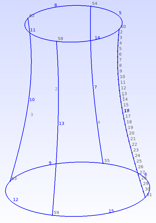
and produces the geometry shown below.

Copied and rotated B-splines.

Sweeping the lines

We are now ready to sweep the lines around the vertical axis of symmetry of the cooling tower.

# Sweep the lines
surf1 = occ.revolve([(1, l1)], 0, 0, 0, 0, 0, 1, math.pi/2)
surf2 = occ.revolve(l2, 0, 0, 0, 0, 0, 1, math.pi/2)
surf3 = occ.revolve(l3, 0, 0, 0, 0, 0, 1, math.pi/2)
surf4 = occ.revolve(l4, 0, 0, 0, 0, 0, 1, math.pi/2)

Swept B-splines.

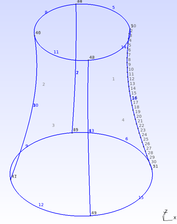
Merging overlapping entities

As you can see for the figure, there are a number of overlapping geometric entities in the figure. We would like to clean that up and merge them. To do that we use the fragment command.

# Join the surfaces
surf5 = occ.fragment(surf1, surf2)
surf6 = occ.fragment(surf3, surf4)
surf7 = occ.fragment(surf5[0], surf6[0])

Merged surfaces.

We are now ready to mesh the geometry after a call to occ.synchronize().

Quadrilateral meshing with gmsh

The most convenient quadrilateral mesh approach in gmsh is to use transfinite interpolation. An example of transfinite interpolation is the Coon’s Patch.

For this approach to work, we need to assign the number of nodes along selected lines.

Circumferential lines

First we set up transfinite interpolation for all the lines, and assign a discretization of 15 nodes for all the lines of the geometry. We will then assign a different number of nodes to the axial lines.

num_nodes_circ = 15
for curve in occ.getEntities(1):
    mesh.setTransfiniteCurve(curve[1], num_nodes_circ)

Axial lines

To match the element density used in the Code-Aster sample mesh, we need 32 nodes along the four lines in the axial direction. We could select these lines using bounding boxes, but in this case it’s more straightforward to just pick the numbers from the gmsh GUI:

num_nodes_vert = 32
vertical_curves = [7, 10, 13, 17]
for curve in vertical_curves:
    mesh.setTransfiniteCurve(curve, num_nodes_vert)

Surfaces

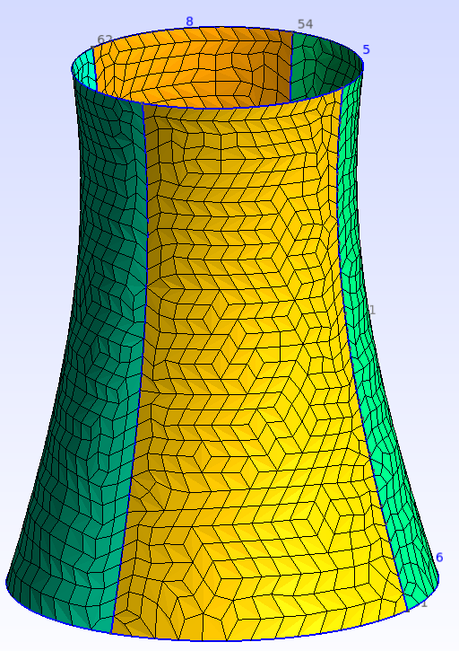
We also need to tell gmsh that the four swept surfaces are transfinite. If we do not, we will get a mesh that looks like the one below.

for surf in occ.getEntities(2):
    mesh.setTransfiniteSurface(surf[1])

Mesh without transfinite surface interpolation

Algorithm and mesh generation

The meshing algorithm settings can now be assigned:

gmsh.option.setNumber('Mesh.RecombineAll', 1)
gmsh.option.setNumber('Mesh.RecombinationAlgorithm', 1)
gmsh.option.setNumber('Mesh.Recombine3DLevel', 2)
gmsh.option.setNumber('Mesh.ElementOrder', 1)

and the mesh generated:

# Generate mesh
mesh.generate(2)

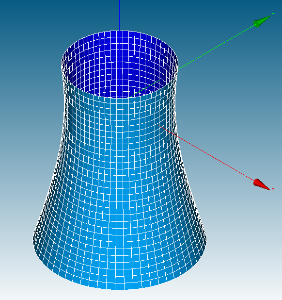
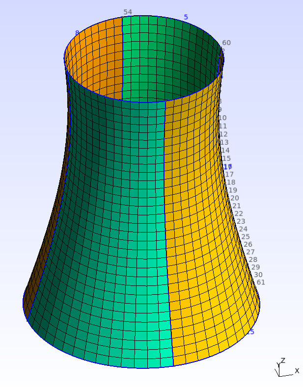
The mesh looks similar to that provided with Code-Aster (and produces almost identical results to the benchmark case):

Quadrilateral mesh

Remarks

This simple procedure can be used to mesh quite complex domains with quadrilateral elements. The other option provided by gmsh for quad meshing is, of code, the extrusion functionality.